Investigating the Optimal Badminton Shuttle Launch Angle
“Finding the optimal angle to land a badminton shuttle in the corner during a service in my school’s badminton court”
Session: May 2025
1.1 Introduction
Badminton is a racket sport played by either two opposing players (singles) or two opposing pairs (doubles), who take positions on opposite halves of a rectangular court that is divided by a net. Players score points by striking a shuttlecock with their racket so that it passes over the net and lands in their opponents' half of the court. A rally ends once the shuttlecock has struck the ground, and the shuttlecock may only be struck once by each side before it passes over the net.
The game is played by a badminton racket made of graphite and a shuttlecock which is a feathered projectile whose unique aerodynamic properties cause it to fly differently from the balls used in most racket sports (Badminton Western Australia). The rally is started by a player launching the feathered shuttle from a starting position known as the serve. Because all players are ready for the shuttle to be launched, the shuttle needs to be served such that the opponent cannot attack immediately: the shuttle should not reach a maximum height more than 15 cm above the net for tactical purposes. Having played badminton for almost 3 years, I have always struggled to serve the shuttle at the perfect height as the opponent is always ready to attack. When preparing for an upcoming badminton tournament I had to find a way to launch the shuttle at the perfect height, speed and angle to improve my chances of making the shuttle land in the corner of the court and make it difficult for my opponent to receive that service.
1.2 Rationale
To understand how to optimize my service and what the “perfect” way is, I decided to use the concepts and skills that I have learnt in my Mathematics Analysis and Approaches HL course. To improve my game and figure out the optimal service, I need to find the optimal combination of the three parameters that I have identified to be affecting my service: initial height, initial velocity and the focus of this exploration: projectile angle.
1.3 Methodology
Primary data, including the ceiling height, badminton net height, and court dimensions will be collected using a measuring tape. A video recording of the service will be used to track the shuttle’s path and measure its initial height using Tracker Pro. The shuttle’s dimensions and surface area will be modeled to calculate air resistance and drag force. Secondary data, such as gravity (9.81 m/s²) and air viscosity, will be sourced from research and data of the locale where the video was taken, including a Purdue University study by Achyut Paudel and Lloyd Smith, which provides drag coefficient, the constant of air resistance, as 0.40. The fluid density of air will be determined using barometric pressure equations. Regression analysis will model the shuttle’s flight path, and arc length calculations will establish the relationship between displacement and time. Using primary and secondary data, mathematical calculations will be performed to determine the optimal launch angle for a “perfect service.”
1.4 Technological Justification
The Tracker Pro application, a video analytics tool, will be used to trace the shuttle’s path, determine the initial height, and measure flight time. Logger Pro will model functions, while all numerical calculations will be performed on a TI Nspire CX II CAS G.D.C. These tools enhance accuracy with flexibility and reliability, though potential errors will be assessed later.
2.0 Calculating the Fluid Density of Air in my Locale
To calculate the fluid density of air, we will first need to calculate the relative atmospheric pressure in my locale. To do this I will be using an existing barometric pressure equation:
$$ P_h = P_0\, e^{-\frac{Mgh}{RT}} \tag{1} $$- \(P_h\) = Atmospheric Pressure at altitude of \(h\)
- \(P_0\) = Atmospheric Pressure at ground level
- \(M\) = Molecular mass of air
- \(g\) = acceleration due to gravity
- \(h\) = altitude of given location
- \(R\) = Universal Gas Constant
- \(T\) = Temperature of area (in Kelvin)
The value for all of the parameters can be collected from secondary data sources. The average annual temperature of my locale is \(20.8\,^\circ\text{C} = 293.95\ \text{K}\). The atmospheric pressure at ground level is considered to be approximately 101,325 Pa (NOAA). The standard molecular mass of air is found to be \(28.95\ \text{g mol}^{-1} = 0.02895\ \text{kg mol}^{-1}\) (Jones). The acceleration due to gravity is \(9.81\ \text{m s}^{-2}\) which is the generally accepted value. The Universal Gas constant is a set value of \(8.3145\ \text{J mol}^{-1}\,\text{K}^{-1}\) (Gregersen). The altitude of my location is approximately \(7{,}200\ \text{feet} = 2200\ \text{m}\). Substituting each of these values in equation (1), we get:
$$ P_h = 101325\, e^{-\frac{(0.02895)(9.81)(2200)}{(8.3145)(293.95)}} = 78436\ \text{Pa} \tag{2} $$After calculating the atmospheric pressure, we must use that to calculate the value of fluid density of air.
$$ \rho_h = \frac{P_h M}{R T} \qquad \text{(fluid density of air at altitude } h) \tag{3} $$Now we can use equation (3) to calculate the numerical value for the fluid density of air at an altitude of 2200 metres.
$$ \rho_h = \frac{(78436)(0.02895)}{(8.3145)(293.95)} = 0.930829\ \text{kg m}^{-3} \tag{4} $$Thus the fluid density of the air in my locale is \(0.930829\ \text{kg m}^{-3}\) with respect to air at ground level.
2.1 Calculating the Horizontal Distance from Service Point to Corner
The dimensions of the badminton court at my school were measured using a measuring tape and are depicted in the figure given below:

Figure 2: Dimensions of the badminton court at my school.
During a service in a singles game, it is strategic for a player to stand at point A and try to serve either B or C. For this exploration, the focus will be on finding the most optimal angle to launch the shuttle from point A to point B. The horizontal distance that the shuttle has to cover is AB. The value for AB can be calculated using the Pythagorean theorem.
$$ a = \sqrt{b^2 + c^2} $$ $$ AB = \sqrt{AD^2 + BD^2} = \sqrt{(1.5+1.5)^2 + 2.6^2} = 3.969\ \text{m} \approx 4\ \text{m} $$2.3 Deriving the Arc-Length Formula to Calculate the Initial Velocity
To calculate the initial velocity of the service, the total arc length of the shuttle’s trajectory must be determined. A video recording of the serve was analyzed using TrackerPro to model the shuttle's path and initial height. Since each service had a unique initial height, averaging would introduce errors, making individual trajectory analysis essential; thus only a single attempt was recorded on video. Using TrackerPro, trajectory points were identified and plotted in Logger Pro for further analysis. A third-degree polynomial was determined to be the best fit for modeling the shuttle’s curved motion, achieving an \(R^2\) (coefficient of determination) value of 0.999. The closer this value is to 1, the more accurate the curve. Table 1 partially presents the data points tracked during the analysis and the rest can be found in Appendix 1B.
Table 1
| x-coordinate | y-coordinate |
|---|---|
| 0.03191856 | 1.19345 |
| 0.5227501 | 1.575907 |
| 1.147597 | 2.090945 |
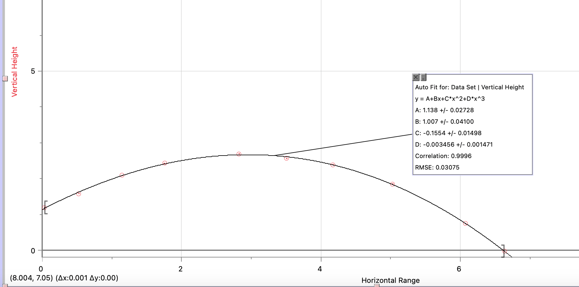
Figure 3: Modeled trajectory of the Shuttle during service
Figure 3 shows the graph of the derived polynomial function using the curve fit function in Logger Pro, which can be simplified by rounding off all coefficients to 3 significant figures. In this function, \(x\) represents the horizontal displacement of the shuttle and the value \(H(x)\) represents the vertical displacement of the shuttle at horizontal displacement \(x\).
$$ H(x) = -0.003456x^3 - 0.1554x^2 + 1.007x + 1.138 \tag{5} $$To find the initial velocity of the shuttle at time \(t = 0\), I will calculate the total distance traveled by calculating the arc length of the function \(H(x)\). Then I will use that to model a function that represents the distance covered for every time interval of 1 second, which can be used to derive a function for the velocity of the shuttle by differentiating the distance with respect to time \(\frac{dL(t)}{dt}\). Considering the function \(H(x)\) and its graph in Figure 3, the length of the arc can be defined as the sum of distances between each point that forms the polynomial function, where the distance between two points on the curve is \(|P_iP_{i+1}|\).
$$ |L| = |P_1P_2| + |P_2P_3| + |P_3P_4| + \cdots + |P_9P_{10}| = \sum_{i=1}^{10} |P_iP_{i+1}| \tag{6} $$However, as my data is limited to only a certain number of points, \(|L|\) might not produce an accurate result. Thus a generalization must be made which accounts for countless intervals, which means that the number of points \(n\) tends to approach infinity.
$$ |L| = \lim_{n \to \infty} \sum_{i=1}^{n} |P_iP_{i+1}| \tag{7} $$Using the distance formula, \(|P_iP_{i+1}|\) can be rewritten in terms of \(x\) and \(H(x)\) as a point on the curve \(P_x = (x, H(x))\).
$$ |P_iP_{i+1}| = \sqrt{(x_{i+1} - x_i)^2 + (H(x_{i+1}) - H(x_i))^2} \tag{8} $$Substituting equation (8) into equation (7), we get a generalisation for \(|L|\):
$$ |L| = \lim_{n \to \infty} \sum_{i=1}^{n} \sqrt{(\Delta x)^2 + (\Delta H(x))^2} \tag{9} $$The Mean Value Theorem (MVT) states that at some point \(c\) in the interval \((a, b)\) the instantaneous rate of change of the function (its derivative) is equal to the average rate of change of the function over \([a, b]\).
$$ f'(c) = \frac{f(b) - f(a)}{b - a} \quad\Longrightarrow\quad f'(x_m) = \frac{\Delta f(x)}{\Delta x} \tag{10} $$We can apply this same concept to the polynomial \(H(x)\) for the point \(x_m \in (x_i, x_{i+1})\) over the interval \([x_i, x_{i+1}]\):
$$ H'(x_m) = \frac{H(x_{i+1}) - H(x_i)}{x_{i+1} - x_i} = \frac{\Delta H(x)}{\Delta x} \quad\Longrightarrow\quad \Delta H(x) = \Delta x\, H'(x_m) \tag{11} $$Substituting the new value of \(\Delta H(x)\) in equation (9), we get:
$$ |L| = \lim_{n \to \infty} \sum_{i=1}^{n} \sqrt{(\Delta x)^2 + (\Delta x\, H'(x_m))^2} \tag{12} $$ $$ |L| = \lim_{n \to \infty} \sum_{i=1}^{n} \sqrt{(\Delta x)^2 (1 + H'(x_m)^2)} = \lim_{n \to \infty} \sum_{i=1}^{n} \Delta x\, \sqrt{1 + H'(x_m)^2} \tag{13} $$A Riemann sum is an approximation of a region's area, obtained by adding up the areas of multiple simplified slices of the region. It is applied in calculus to formalize the method of exhaustion, used to determine the area of a region. This process yields the integral, which computes the value of the area exactly as shown in the equation below (Brilliant).
$$ \int_a^b f(x)\, dx = \lim_{n \to \infty} \sum_{i=1}^{n} f(x_i)\, \Delta x \tag{14} $$We can convert our expression of \(|L|\) into a definite integral between the limits \((a, b)\), which in this case will be the \(x\)-coordinate of the initial point on the polynomial \(H(x)\) and the \(x\)-coordinate of the final point on the polynomial \(H(x)\).
$$ |L| = \int_a^b \sqrt{1 + H'(x_m)^2}\, dx \tag{15} $$To find the value of \(H'(x)\), we must differentiate the function \(H(x)\):
$$ H(x) = -0.003456x^3 - 0.1554x^2 + 1.007x + 1.138 $$ $$ \frac{d}{dx}H(x) = -0.010368x^2 - 0.3108x + 1.007 \tag{16} $$Upper bound \(= 6.631229\) (maximum horizontal distance covered)
Lower bound \(= 0.03191856\) (starting horizontal position)
Substituting equation (16) into equation (15) we get the following:
$$ |L| = \int_{0.03191856}^{6.631229} \sqrt{1 + (-0.010368x^2 - 0.3108x + 1.007)^2}\, dx = 8.1041 \approx 8.1\ \text{m} $$Now that the arc length is calculated, the value can be used to determine the initial velocity of the shuttle. To do this, we have to calculate how much time the shuttle takes to cover 1 m of horizontal displacement. This can be done by calculating the ratio of horizontal displacement versus time. We earlier found the maximum horizontal displacement to be 6.63 m and the time taken to be 1.134 s.
$$ \text{Ratio of } h \text{ vs } t = \frac{t}{h} = \frac{1.134}{8.1041} \approx 0.139929 \tag{17} $$Therefore for every horizontal metre the shuttle was displaced, approximately 0.1454 seconds passed. The next step is to calculate the length of the arc for each metre covered. We will be using the following functions to calculate the arc length for every horizontal displacement value and the time taken to cover \(x\) metres. If the shuttle travelled \(x\) metres, the arc length for its previous one metre covered will be the following integral with limits \(x\) and \(x-1\):
$$ L(x) = \int_{x-1}^{x} \sqrt{1 + (-0.010368x^2 - 0.3108x + 1.007)^2}\, dx, \qquad 0 < x \le 7 \tag{18} $$ $$ T(x) = 0.139929\, x \tag{19} $$For example:
$$ T(1) = 0.139929 \cdot 1 = 0.139929 $$ $$ L(1) = \int_{0}^{1} \sqrt{1 + (-0.010368x^2 - 0.3108x + 1.007)^2}\, dx = 1.31315 $$Thus, we can create a table comparing the time period, horizontal displacement and the arc length:
Table 2
| Horizontal Distance \(x\) | Time taken \(T(x)\) | Arc Length \(L(x)\) |
|---|---|---|
| 1 | 0.139929 | 1.31315 |
| 2 | 0.279858 | 2.44213 |
| 3 | 0.419787 | 3.46079 |
| 4 | 0.559716 | 4.48805 |
| 5 | 0.699645 | 5.65976 |
| 6 | 0.839574 | 7.08858 |
| 7 | 0.979503 | 8.85322 |
However, to find the velocity curve of the shuttle, we need to establish a relationship between the arc-length \(L(x)\) of the shuttle and the time period \(T(x)\). This can be done by plotting the time period on the \(x\)-axis and the arc length on the \(y\)-axis. The second and third columns from Table 2 can be used as input to generate a graph in Logger Pro. After plotting the graph, I was able to use Logger Pro’s Curve Fit function once again to generate a polynomial function \(L(t)\), and a quartic curve had a correlation of 1 which was the greatest. Thus the following represents the curve \(L(t)\) and helps us derive a polynomial expression for it.
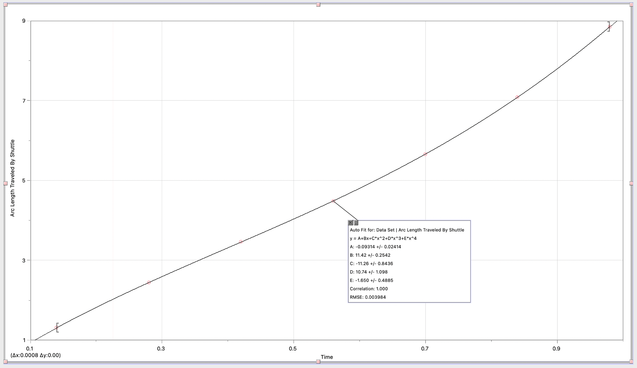
Figure 4: Polynomial Fit for the arc length curve
When using the curve fit function, I found that the polynomial of best fit had a degree of 4. The polynomial function that was identified is the following:
$$ L(t) = -1.650t^4 + 10.74t^3 - 11.26t^2 + 11.42t - 0.093 \tag{20} $$To derive a polynomial for the velocity of the shuttle, the function \(L(t)\) can be differentiated with respect to \(t\), as it is an established mathematical relation that differentiating distance with respect to time gives velocity.
$$ V(t) = \frac{d}{dt}L(t) = -4(1.650)t^3 + 3(10.74)t^2 - 2(11.26)t + 11.42 \tag{21} $$ $$ V(t) = -6.6t^3 + 32.33t^2 - 22.52t + 11.42 \tag{22} $$Now that we have a polynomial that represents the velocity of the shuttle for every time period, we can calculate the initial velocity by evaluating \(V(t)\) at \(t = 0\):
$$ V(0) = -6.6(0)^3 + 32.33(0)^2 - 22.52(0) + 11.42 = 11.42 \tag{23} $$Therefore: initial velocity \((u) = 11.42\ \text{m s}^{-1}\).
2.4 Resolving Velocity into its Vector Components
Because velocity is a vector quantity, we can split velocity into horizontal and vertical velocity, which indicate the magnitude with which the object is moving vertically or horizontally. This can be done by using the angle of deviation from the \(x\)-axis as \(\theta\). The horizontal component of velocity can be represented as \(v\cos\theta\) and the vertical component of velocity can be represented as \(v\sin\theta\). Figure 5 displays this effect visually.
Figure 5: Resolving velocity into vector components
2.5 Calculating the Effect of Drag Force
During the flight of the shuttle, there are multiple forces acting on the shuttle. Until now we have explored the effect of gravity through the curved trajectory of the projectile. However, due to this being a real-life application, we have to also account for the effect of drag force (air resistance) on the shuttle’s flight. To see how the forces act on the shuttle, we can draw a free body diagram of the shuttle mid-flight.
Figure 6: Free body diagram of the shuttle mid-flight
In Figure 6 we see the different forces acting on the shuttle. There is the force of gravity, acting downwards with a magnitude of \(mg\). However there is also drag force, which acts opposite to the direction of motion with a magnitude of \(d\) and at an angle of \(\theta\). Like we had resolved velocity into directional vector components, we can do the same here by resolving the drag force as \(-d\sin\theta\) for the vertical component and \(-d\cos\theta\) for the horizontal component. The following formula helps us calculate drag force \((d)\), where \(C\) is the drag coefficient, \(A\) is the surface area of the object exposed to the air, \(v\) is the velocity and \(\rho\) is the fluid density of air.
$$ d = \tfrac{1}{2} C \rho v^2 A \tag{24} $$One limiting factor here could be a lack of diversity in the collected data, as for this exploration I am performing all calculations on a Yonex Mavis 350 shuttle, which has specific dimensions and weight, as changes in weight and surface area can affect the amount of drag force experienced. While it restricts the scope of the exploration, using a singular shuttle enables the calculations to be consistent, as the following calculations factor in the exact dimensions of the shuttle. Our biggest calculation is the surface area of the shuttle. Firstly, we can use Logger Pro’s Curve Fit function to map out the outline of the shuttle’s dimensions that are properly calibrated to the graph.
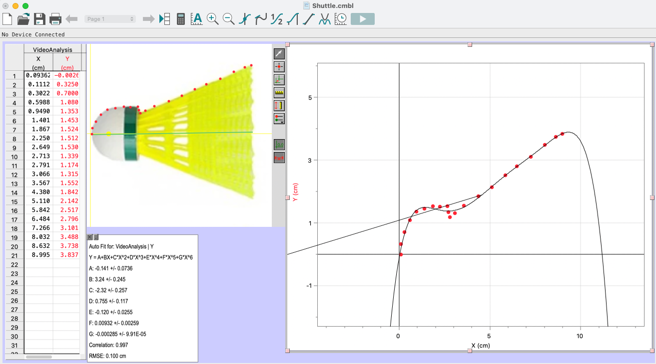
Figure 7: Modeling the outline of the shuttle
After trying various degrees of polynomials, I figured out that a polynomial function of degree 6 had the least amount of standard deviation and the highest value of \(R^2\) for accuracy in modelling. Thus using the numerous points plotted, I was able to arrive at the following polynomial (with 3 significant figures):
$$ f(x) = -2.85 \times 10^{-4} x^6 + 9.32 \times 10^{-3} x^5 - 0.12 x^4 + 0.755 x^3 - 2.32 x^2 + 3.24 x - 0.141 \tag{25} $$To calculate the outer surface area of the shuttlecock, I will be using the following formula for the surface area of revolution for this function, which I took from the Indian Institute of Technology Kanpur’s public calculus class material:
$$ A = \int_a^b 2\pi f(x) \sqrt{1 + (f'(x))^2}\, dx \tag{26} $$To use this formula, we must derive \(f'(x)\), which can be done by differentiating \(f(x)\):
$$ f'(x) = -6(2.85 \times 10^{-4})x^5 + 5(9.32 \times 10^{-3})x^4 - 4(0.12)x^3 + 3(0.755)x^2 - 2(2.32)x + 3.24 $$ $$ f'(x) = -17.1 \times 10^{-4} x^5 + 46.6 \times 10^{-3} x^4 - 0.48 x^3 + 2.265 x^2 - 4.64 x + 3.24 \tag{27} $$The \(x\)-coordinates of the first and last point mapped on the graph in Figure 7 can be taken as the upper and lower bounds \([a, b]\).
Lower bound \(a = 0\)
Upper bound \(b = 8.995\)
The G.D.C. was not able to compute such a large integral, and thus a piece of computer code written in Python (shown in Appendix 1A) was used to calculate the value of \(A\).
However, one limitation that can be observed is the pattern of the shuttle’s surface, which includes a mesh-like structure and 16 triangular gaps. To overcome this limitation, I will be calculating the surface area of each triangular gap and summing it, then subtracting it from the initial left half of the surface area of the shuttle. For the other half, right of the triangular gaps, I will consider the surface area to be half the calculated area due to the mesh-like structure. Considering that \(a_n\) represents the area of the \(n\)th triangular gap, when the gaps exist between the interval \([c, d]\), we can rewrite the expression of \(A\) as the following formula:
$$ A = 2\int_a^b \pi f(x) \sqrt{1 + (f'(x))^2}\, dx - \sum_{n=1}^{16} a_n - \int_d^b \pi f(x) \sqrt{1 + (f'(x))^2}\, dx \tag{29} $$The first step to calculate the surface area of the triangular gaps is to get their exact dimensions, which can be done using Logger Pro’s photo analysis software. To do this, I will use the calibrated measurement tool to calculate the length of the sides of the triangle. Then I will mark the points for the intervals \([c, d]\) and \([d, b]\).
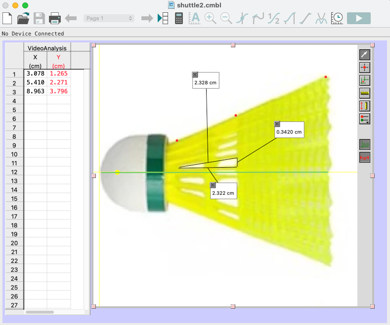
Figure 8: Calculating dimensions of Triangular Gaps
Dimensions calculated:
- side 1 of \(\triangle\) = 2.32 cm
- side 2 of \(\triangle\) = 2.32 cm
- side 3 of \(\triangle\) = 0.34 cm
- \(c\) at \(x = 3.078\) cm
- \(d\) at \(x = 5.410\) cm
- \(b\) at \(x = 8.96\) cm
To calculate the area of each triangular gap I will be using Heron’s Formula, as all three sides are known:
$$ s = \frac{\text{side}_1 + \text{side}_2 + \text{side}_3}{2} = \frac{2.32 + 2.32 + 0.34}{2} = 2.49\ \text{cm} \tag{30} $$ $$ a_n = \sqrt{s(s-a)(s-b)(s-c)} \tag{31} $$ $$ a_n = \sqrt{2.49(2.49 - 2.32)(2.49 - 2.32)(2.49 - 0.34)} \approx 0.39\ \text{cm}^2 \tag{32} $$Now we can calculate the adjusted surface area using the following expression:
$$ A = 2\int_a^b \pi f(x) \sqrt{1 + (f'(x))^2}\, dx - \sum_{n=1}^{16} a_n - \int_d^b \pi f(x) \sqrt{1 + (f'(x))^2}\, dx \tag{33} $$ $$ A = 121.172206 - \sum_{n=1}^{16}(0.39) - \int_{5.410}^{8.96} \pi f(x) \sqrt{1 + (f'(x))^2}\, dx \tag{34} $$ $$ A = 121.172206 - 6.24 - 32.253077 = 82.6791\ \text{cm}^2 \approx 0.00827\ \text{m}^2 $$After getting the value for surface area, we can calculate the drag force, as we know the drag coefficient \((C)\) to be 0.40, the air density to be \(0.930829\ \text{kg m}^{-3}\), and the velocity to be \(v\). Thus:
$$ d = \tfrac{1}{2} C \rho v^2 A = \tfrac{1}{2}(0.40)(0.930829)(11.42)^2(0.00827) \tag{35} $$ $$ d = 0.401576 \approx 0.4\ \text{N} $$Newton’s second law defines a force to be equal to the change in momentum (mass times velocity) per change in time. Momentum is defined to be the mass \(m\) of an object times its velocity \(v\).
$$ \text{momentum } (p) = mv \tag{36} $$ $$ F = \frac{\Delta p}{\Delta t} = \frac{m\,\Delta v}{\Delta t} \tag{37} $$In the current scenario, there is no change in mass:
$$ F = \frac{m\,\Delta v}{\Delta t} = m\frac{dv}{dt} = ma \tag{38} $$To calculate the acceleration in the direction opposite to air resistance, we take \(F = d\):
$$ F = ma \quad\Longrightarrow\quad a = \frac{F}{m} = \frac{d}{m} \tag{39} $$The mass of the shuttle \((m)\) was measured to be 0.03 kg. Thus we can calculate the acceleration \((a)\):
$$ a = \frac{0.4}{0.03} = 13.33\ \text{m s}^{-2} $$2.6 Deriving Projectile Motion Equations
The acceleration \((a)\) that I previously calculated can be divided into its vector components. The horizontal component is \(a_x = a\cos\theta\) and the vertical component is \(a_y = a\sin\theta\). However, as this acceleration is acting opposite to the line of motion, we take \(a_x = -a\cos\theta\) and \(a_y = -a\sin\theta\). Additionally, gravitational force is acting on the shuttle too, and as it always acts vertically downwards, we simply add \(g\) to the vertical component:
$$ a_x = -a\cos\theta \tag{40} $$ $$ a_y = -a\sin\theta - g \tag{41} $$Using these components we can calculate the loss in horizontal and vertical velocity, which we had resolved earlier in section 2.4. Because differentiating velocity gives us acceleration (as it is the rate of change of velocity), integrating acceleration should give us velocity. Applying the same logic, we can integrate the vector components of acceleration to get a value for the vector components of velocity.
$$ v_x = v\cos\theta - \int a\cos\theta\, dt = v\cos\theta - at\cos\theta \tag{42} $$ $$ v_y = v\sin\theta - \int (a\sin\theta + g)\, dt = v\sin\theta - at\sin\theta - gt \tag{43} $$Equations (42) and (43) are both first-order equations and are part of a single vector quantity \(v\). They can be represented as follows:
$$ x = \int \frac{dx}{dt}\, dt = \int v_x\, dt = \int (v\cos\theta - at\cos\theta)\, dt \tag{44} $$ $$ x = vt\cos\theta - \tfrac{1}{2}at^2\cos\theta + C \tag{45} $$ $$ y = \int \frac{dy}{dt}\, dt = \int v_y\, dt = \int (v\sin\theta - at\sin\theta - gt)\, dt \tag{46} $$ $$ y = vt\sin\theta - \tfrac{1}{2}at^2\sin\theta - \tfrac{1}{2}gt^2 + C \tag{47} $$Because at \(t = 0\), horizontal distance \(x = 0\):
$$ x = 0 - 0 + C \Longrightarrow C = 0 $$ $$ x = vt\cos\theta - \tfrac{1}{2}at^2\cos\theta \tag{48} $$Because at \(t = 0\), the vertical distance (the initial height of the shuttle) \(y = 1.19345\) m:
$$ y = 0 - 0 - 0 + C \Longrightarrow C = 1.19345 $$ $$ y = vt\sin\theta - \tfrac{1}{2}at^2\sin\theta - \tfrac{1}{2}gt^2 + 1.19345 \tag{49} $$2.7 Calculating the Optimal Angle
We already found that for a corner serve, the horizontal distance to be covered is 4 m. We also found the time at which the shuttle lands on the ground to be \(t\). We also used the arc length to calculate the initial velocity \((v)\), and finally we calculated the value for acceleration \((a)\). As \(\theta\) is a constant value set at launch, we can use the variable \(t\) to calculate \(\theta\). When \(x = 4\) m:
$$ x = vt\cos\theta - \tfrac{1}{2}at^2\cos\theta = \cos\theta\left(vt - \tfrac{1}{2}at^2\right) \tag{50} $$ $$ \frac{x}{vt - \tfrac{1}{2}at^2} = \cos\theta \quad\Longrightarrow\quad \theta = \cos^{-1}\!\left(\frac{x}{vt - \tfrac{1}{2}at^2}\right) \tag{51} $$However, recalling that due to tactical reasons the maximum vertical displacement is 1.70 m:
$$ y \le 1.70 $$ $$ vt\sin\theta - \tfrac{1}{2}at^2\sin\theta - \tfrac{1}{2}gt^2 + C \le 1.70 \tag{52} $$ $$ \sin\theta\left(vt - \tfrac{1}{2}at^2\right) \le 1.70 + \tfrac{1}{2}gt^2 - C $$ $$ \theta \le \sin^{-1}\!\left(\frac{1.70 + \tfrac{1}{2}gt^2 - C}{vt - \tfrac{1}{2}at^2}\right) \tag{53} $$However, to avoid the shuttle hitting the net, the minimum height has to be the sum of the height of the net (1.5 m) and the diameter of the shuttle (0.0751 m), which is:
$$ H_{min} = 1.5 + 0.0751 = 1.5751\ \text{m} \tag{54} $$Therefore,
$$ \sin^{-1}\!\left(\frac{1.5751 + \tfrac{1}{2}gt^2 - C}{vt - \tfrac{1}{2}at^2}\right) \le \theta \le \sin^{-1}\!\left(\frac{1.70 + \tfrac{1}{2}gt^2 - C}{vt - \tfrac{1}{2}at^2}\right) \tag{55} $$Substituting the values for \(x\), \(v\), \(t\), \(g\), \(a\), we can calculate \(\theta\) with \(x = 1\) m and \(t = T(x) = 0.139929\) (taken from Table 2):
$$ \sin^{-1}\!\left(\frac{1.5751 + \tfrac{1}{2}(9.81)(0.139929)^2 - 1.19345}{(11.42)(0.139929) - \tfrac{1}{2}(13.33)(0.139929)^2}\right) \le \theta \le \sin^{-1}\!\left(\frac{1.70 + \tfrac{1}{2}(9.81)(0.139929)^2 - 1.19345}{(11.42)(0.139929) - \tfrac{1}{2}(13.33)(0.139929)^2}\right) \tag{56} $$ $$ 18.9968^\circ \le \theta \le 24.2442^\circ \tag{57} $$Thus the most optimal angle to launch the shuttle into the short corner in my locale and setting was found to be between 18.9 and 24.2 degrees. (Applicable only to Yonex Mavis 350 shuttles.)
3.1 Evaluation: Strengths of the Exploration
- All secondary data collected, including formulae, laws and constants, have been taken from reliable sources such as university lectures, research articles and research papers.
- The use of regression analysis helps minimize outliers and errors.
- The same apparatus and environment has been used throughout the exploration, which helps keep the data consistent and all calculations easy to perform.
3.2 Evaluation: Limitations of the Exploration
Besides the limitations discussed throughout the calculations, there are a few more I observed:
- The value for air resistance derived is highly simplified, as there are multiple factors that come into play like the angle of motion and the rotation and revolution of the shuttle.
- The results of this exploration apply only in the settings in my locale and school building, as parameters such as temperature, elevation, air density, and court dimensions change from place to place, which reduces the scope for generalisation.
- We have assumed that the initial velocity of the shuttle remains constant. However this is rather unrealistic, as it is humanly impossible to consistently serve with constant velocity.
- All calculations have been done with 3 significant figures, which reduces accuracy.
3.3 Evaluation: Possibilities for Further Exploration
If I had more time to explore this topic, I would have explored how the air resistance of the shuttle changes with the amount of spin and angle. This is because over the past year I have learnt the ability to give the shuttle some spin and rotation, and when I do so, I have observed that the shuttle flies smoother and suddenly dips. This creates unpredictability and I want to study that so I can better understand the fluid dynamics and how it works. This extension could also help me improve my game and understand what my opponent might try and do. I would also like to perform this exploration in different settings, courts and with different shuttles that have different dimensions and surfaces. This would help me generalise my results further and improve my chances at predicting the path of the shuttle. I would also like to perform this exploration for different locations on the badminton court, like the corners at the far back and a perfect net serve (a serve where the shuttle hits a small part of the net before crossing, making it unpredictable and harder to receive).
3.4 Conclusion
As seen in section 2.7, the most optimal angle to launch a short corner serve in my setting with a Yonex Mavis 350 plastic shuttle was found to be between 18.9 and 24.2 degrees. This exploration has provided me with great insight into how I can improve my game. I hope to use this knowledge to condition my muscles and adjust my technique to land a “perfect” corner serve almost every time. This exploration has proved itself to be a valuable learning experience, allowing me to explore many different topics such as differentiation, integration, vectors and graphical modelling. I gained a lot of new knowledge from differentiation, such as the area of revolution formula and the definition of the integral, which helped me connect limits with integration. Moreover, it helped me deepen my knowledge of projectile motion, vectors and mechanics, which I have been learning and using in my IBDP Physics HL class. This exploration proved to be an insightful way for me to link my knowledge between my Physics HL and Mathematics HL classes.
4.0 Bibliography
- Badminton Western Australia. “About the Game: Badminton WA.” Www.badmintonwa.org.au, 2022, www.badmintonwa.org.au/where-play/about-game.
- Brilliant. “Riemann Sums | Brilliant Math & Science Wiki.” Brilliant.org, 2019, brilliant.org/wiki/riemann-sums/.
- Chapter 2. Atmospheric Pressure 2.1 Measuring Atmospheric Pressure.
- Gregersen, Erik. “Boltzmann Constant | Physics.” Encyclopædia Britannica, 2019, www.britannica.com/science/Boltzmann-constant.
- ———. “Ideal Gas Law | Definition, Formula, & Facts | Britannica.” Www.britannica.com, 22 Feb. 2023, www.britannica.com/science/ideal-gas-law.
- Jones, F.E. “The Air Density Equation and the Transfer of the Mass Unit.” Journal of Research of the National Bureau of Standards, vol. 83, no. 5, Sept. 1978, p. 419, https://doi.org/10.6028/jres.083.028.
- Kodaikanal | Dindigul District | India. dindigul.nic.in/tourist-place/kodaikanal/.
- NOAA. “Air Pressure.” Www.noaa.gov, 24 Mar. 2023, www.noaa.gov/jetstream/atmosphere/air-pressure.
5.1 Appendix 1A
import numpy as np
from scipy.integrate import quad

# Define the integrand function
def integrand(x):
    return (
        (-2.85e-4 * x**6
         + 9.32e-3 * x**5
         - 0.12 * x**4
         + 0.755 * x**3
         - 2.32 * x**2
         + 3.24 * x
         - 0.141)
        * np.sqrt(
            1
            + (-17.1e-4 * x**5
               + 46.6e-3 * x**4
               - 0.48 * x**3
               + 2.265 * x**2
               - 4.64 * x
               + 3.24)**2
        )
    )

result, error = quad(integrand, 0, 8.995)
amplitude = 2 * np.pi * result
print(f"Amplitude (A): {amplitude:.6f} cm^2")
print(f"Estimated error in integration: {error:.6e}")


# Output:
# Amplitude (A): 121.172206 cm^2
# Estimated error in integration: 2.261971e-08
5.2 Appendix 1B
| x-coordinate | y-coordinate |
|---|---|
| 0.03191856 | 1.19345 |
| 0.5227501 | 1.575907 |
| 1.147597 | 2.090945 |
| 1.756677 | 2.428332 |
| 2.824498 | 2.689196 |
| 3.505165 | 2.567045 |
| 4.170702 | 2.385731 |
| 5.02687 | 1.847918 |
| 6.072554 | 0.7462548 |
| 6.631229 | 0 |